Example Cases

Lax shock tube problem (1D)

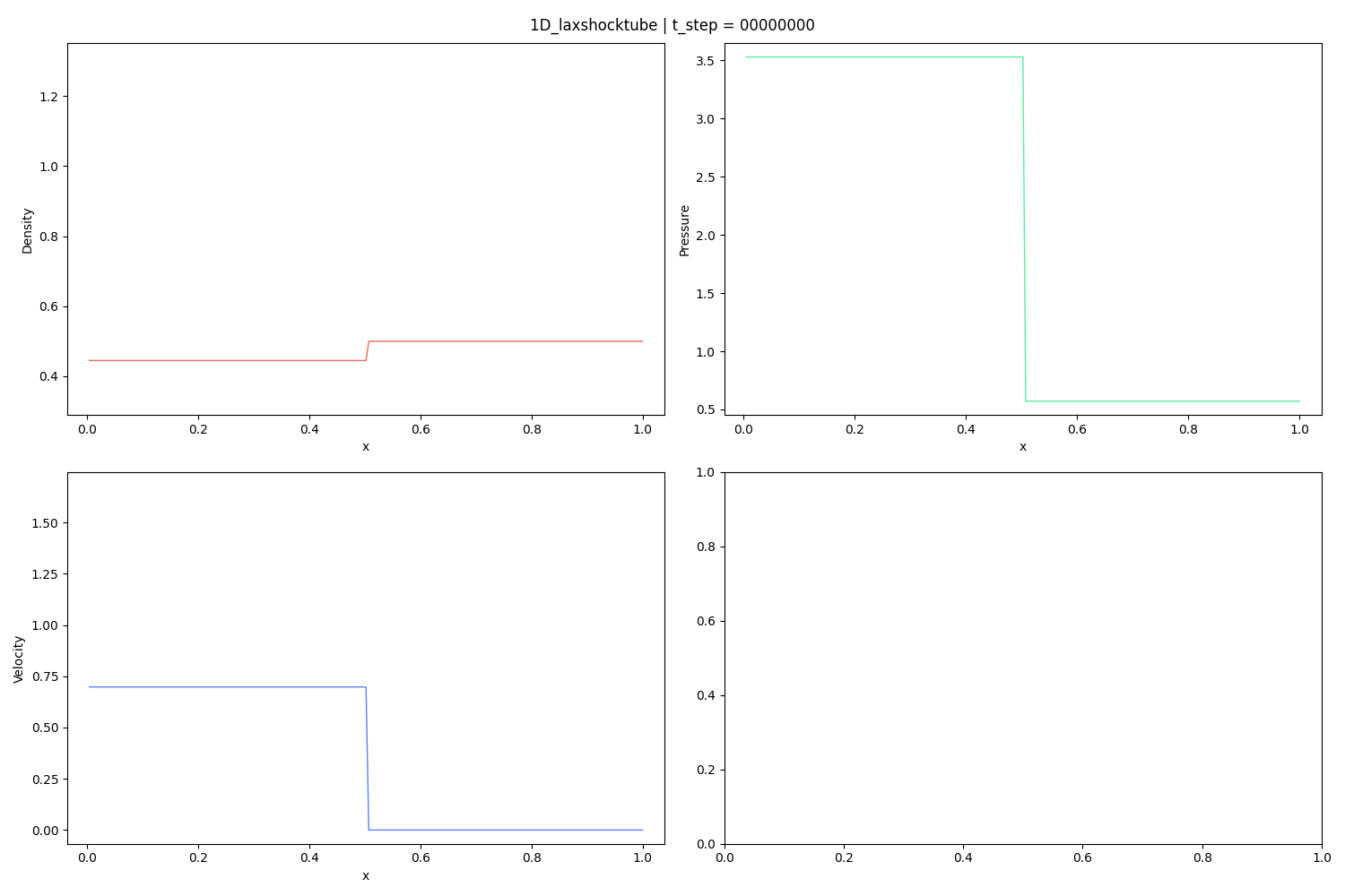
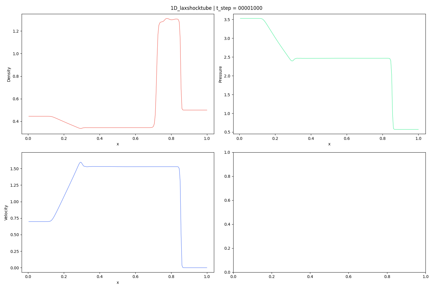
Reference:

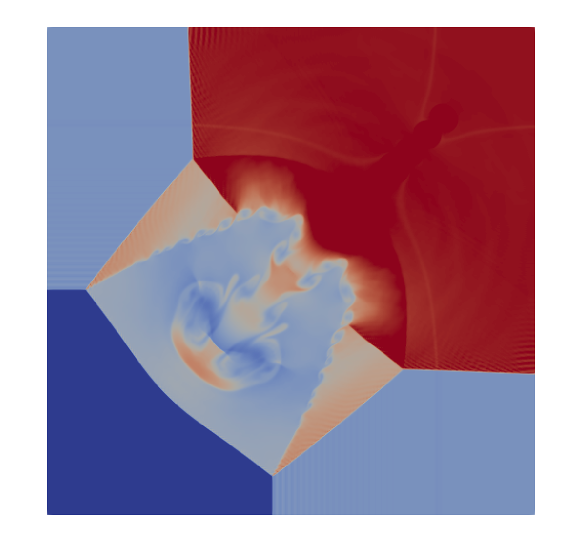
P. D. Lax, Weak solutions of nonlinear hyperbolic equations and their numerical computation, Communications on pure and applied mathematics 7 (1) (1954) 159–193.

Initial Condition

Result

Scaling and Performance test

The scaling case can exercise both weak- and strong-scaling. It adjusts itself depending on the number of requested ranks.

This directory also contains a collection of scripts used to test strong and weak scaling on OLCF Frontier.

Weak Scaling

Pass --scaling weak. The --memory option controls (approximately) how much memory each rank should use, in Gigabytes. The number of cells in each dimension is then adjusted according to the number of requested ranks and an approximation for the relation between cell count and memory usage. The problem size increases linearly with the number of ranks.

Strong Scaling

Pass --scaling strong. The --memory option controls (approximately) how much memory should be used in total during simulation, across all ranks, in Gigabytes. The problem size remains constant as the number of ranks increases.

Example

For example, to run a weak-scaling test that uses ~4GB of GPU memory per rank on 8 2-rank nodes with case optimization, one could:

./mfc.sh run examples/scaling/case.py -t pre_process simulation                    \
             -e batch -p mypartition -N 8 -n 2 -w "01:00:00" -# "MFC Weak Scaling" \
             --case-optimization -j 32 -- --scaling weak --memory 4

Rayleigh-Taylor Instability (3D)

Final Condition and Linear Theory

2D IBM CFL dt (2D)

Result

Shu-Osher problem (1D)

Reference:

C. W. Shu, S. Osher, Efficient implementation of essentially non-oscillatory shock-capturing schemes, Journal of Computational Physics 77 (2) (1988) 439–471. doi:10.1016/0021-9991(88)90177-5.

Initial Condition

Result

Kelvin-Helmholtz Instability (2D)

Reference: See Example 4.8.

A.S. Chamarthi, S.H. Frankel, A. Chintagunta, Implicit gradients based novel finite volume scheme for compressible single and multi-component flows, arXiv preprint arXiv:2106.01738 (2021).

Initial State

Evolved State

Gas Jet (2D)

Final Condition

1D Multi-Component Reactive Shock Tube

References:

P. J. Martínez Ferrer, R. Buttay, G. Lehnasch, and A. Mura, “A detailed verification procedure for compressible reactive multicomponent Navier–Stokes solvers”, Computers & Fluids, vol. 89, pp. 88–110, Jan. 2014. Accessed: Oct. 13, 2024. [Online]. Available: https://doi.org/10.1016/j.compfluid.2013.10.014

H. Chen, C. Si, Y. Wu, H. Hu, and Y. Zhu, “Numerical investigation of the effect of equivalence ratio on the propagation characteristics and performance of rotating detonation engine”, Int. J. Hydrogen Energy, Mar. 2023. Accessed: Oct. 13, 2024. [Online]. Available: https://doi.org/10.1016/j.ijhydene.2023.03.190

Initial Condition

Results

Forward Facing Step (2D)

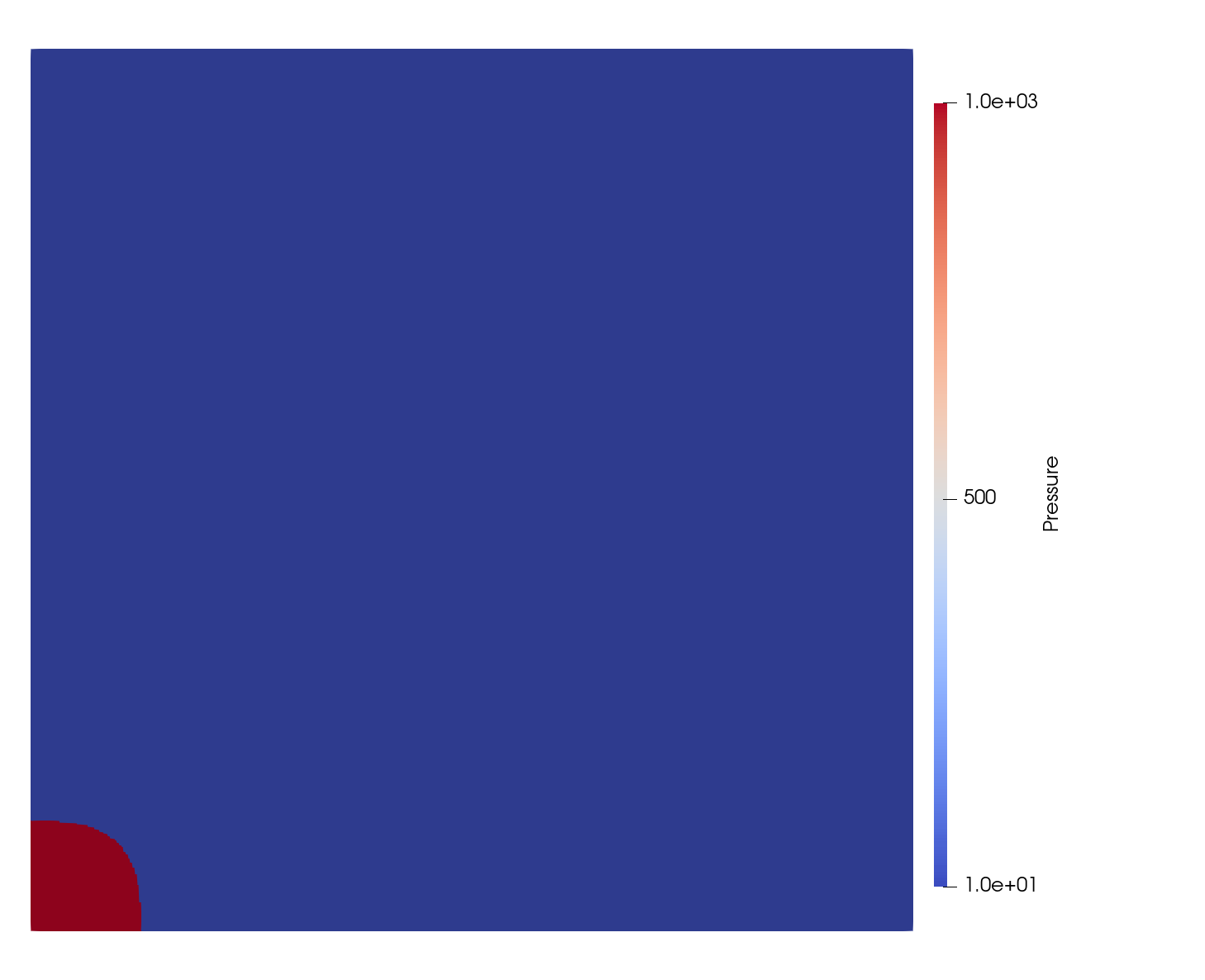
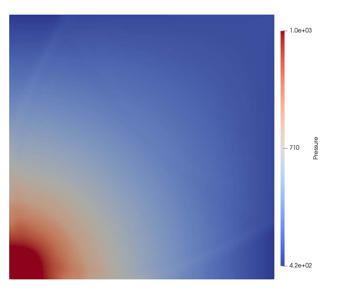
Reference:

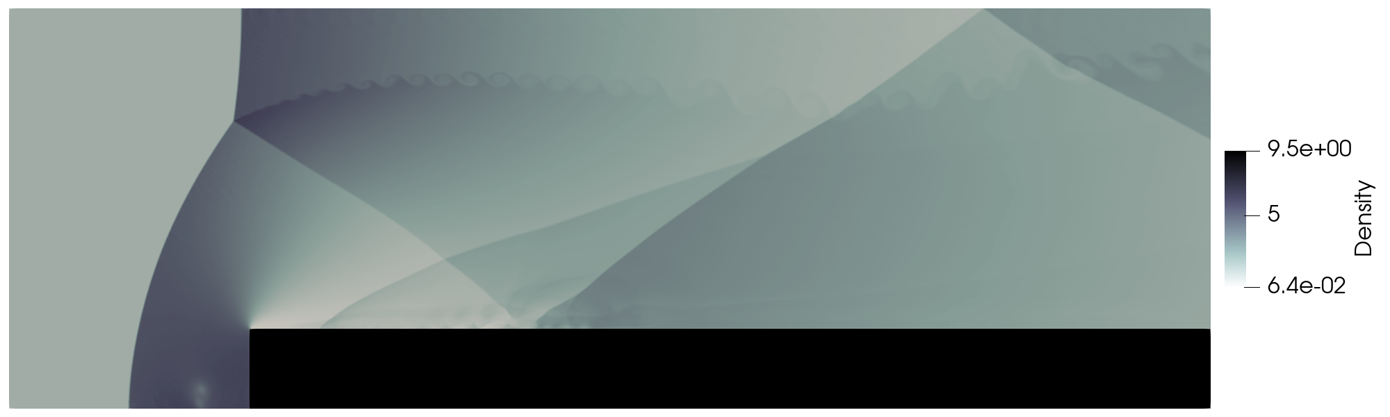
Woodward, P. (1984). The numerical simulation of two-dimensional fluid flow with strong shocks. Journal of Computational Physics, 54(1), 115–173. https://doi.org/10.1016/0021-9991(84)90140-2

Final Condition (Density)

2D Riemann Test (2D)

Reference:

Chamarthi, A., & Hoffmann, N., & Nishikawa, H., & Frankel S. (2023). Implicit gradients based conservative numerical scheme for compressible flows. arXiv:2110.05461

Density Initial and Final Conditions

Perfectly Stirred Reactor

Reference:

G. B. Skinner and G. H. Ringrose, “Ignition Delays of a Hydrogen—Oxygen—Argon Mixture at Relatively Low Temperatures”, J. Chem. Phys., vol. 42, no. 6, pp. 2190–2192, Mar. 1965. Accessed: Oct. 13, 2024.

$ python3 analyze.py
Induction Times ([OH] >= 1e-6):
 + Skinner et al.: 5.200e-05 s
 + Cantera:        5.130e-05 s
 + (Che)MFC:       5.130e-05 s

Lid-Driven Cavity Problem (2D)

Reference:

Bezgin, D. A., & Buhendwa A. B., & Adams N. A. (2022). JAX-FLUIDS: A fully-differentiable high-order computational fluid dynamics solver for compressible two-phase flows. arXiv:2203.13760

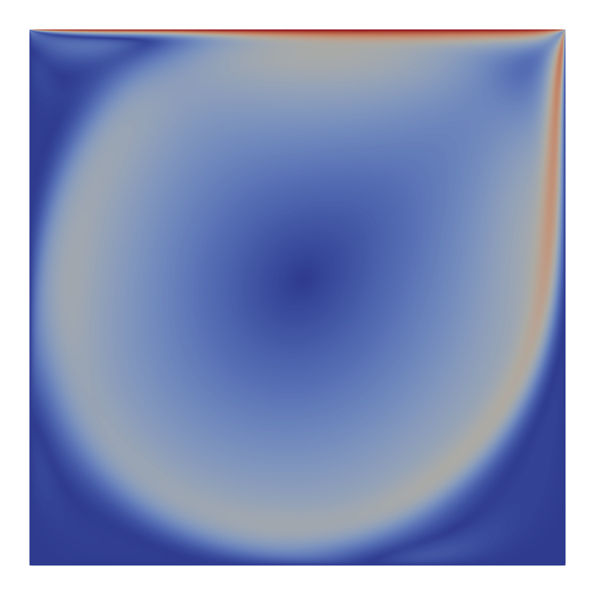
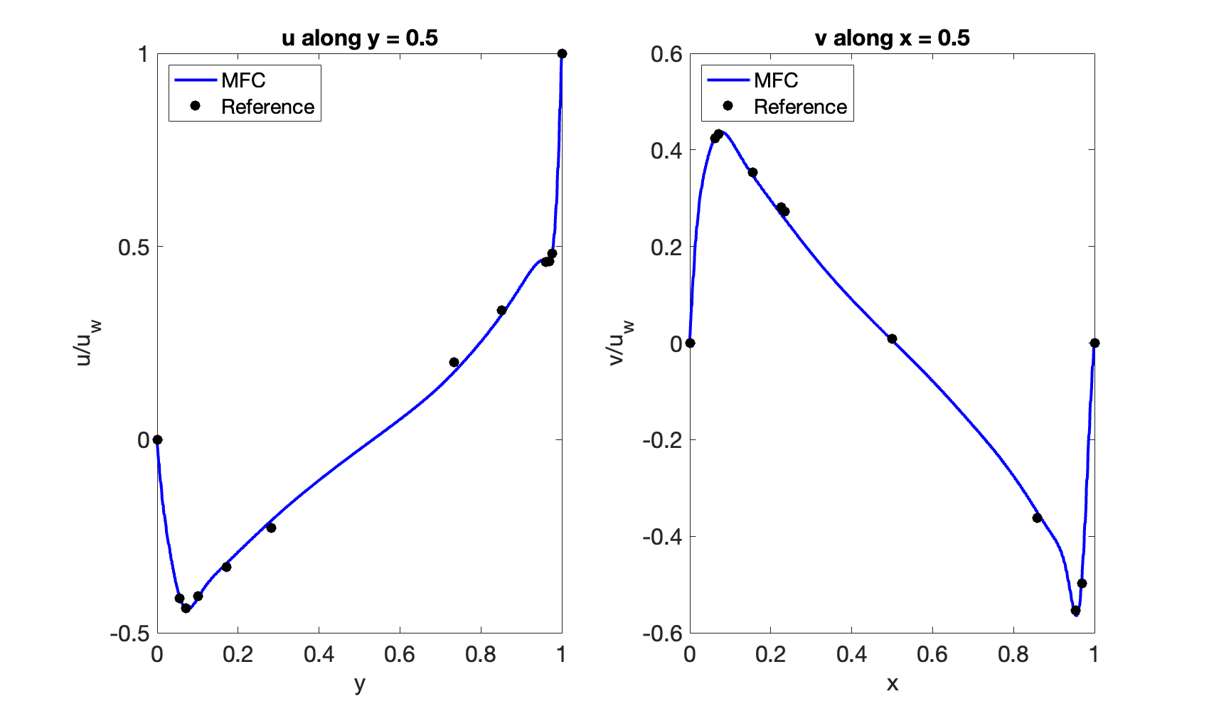
Ghia, U., & Ghia, K. N., & Shin, C. T. (1982). High-re solutions for incompressible flow using the Navier-Stokes equations and a multigrid method. Journal of Computational Physics, 48, 387-411

Final Condition

Centerline Velocities

Richtmyer-Meshkov Instability (2D)

Reference: See Example 4.18.

A.S. Chamarthi, S.H. Frankel, A. Chintagunta, Implicit gradients based novel finite volume scheme for compressible single and multi-component flows, arXiv preprint arXiv:2106.01738 (2021).

Initial State

Evolved State

Viscous Shock Tube (2D)

Reference: See Example 4.13.

A.S. Chamarthi, S.H. Frankel, A. Chintagunta, Implicit gradients based novel finite volume scheme for compressible single and multi-component flows, arXiv preprint arXiv:2106.01738 (2021)., see Example 4.13

Initial State

Evolved State

Isentropic vortex problem (2D)

Reference:

Coralic, V., & Colonius, T. (2014). Finite-volume Weno scheme for viscous compressible multicomponent flows. Journal of Computational Physics, 274, 95–121. https://doi.org/10.1016/j.jcp.2014.06.003

Density

Density Norms

Titarev-Toro problem (1D)

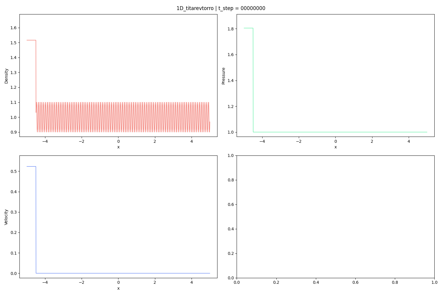
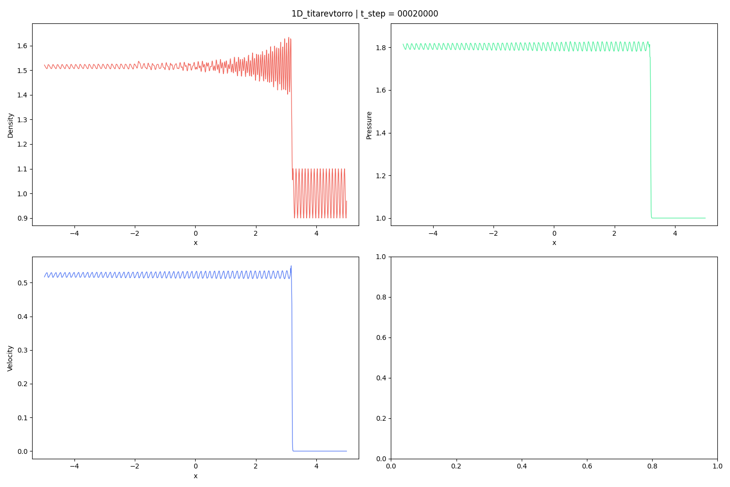
Reference:

V. A. Titarev, E. F. Toro, Finite-volume WENO schemes for three-dimensional conservation laws, Journal of Computational Physics 201 (1) (2004) 238–260.

Initial Condition

Result

2D Hardcodied IC Example

Initial Condition and Result

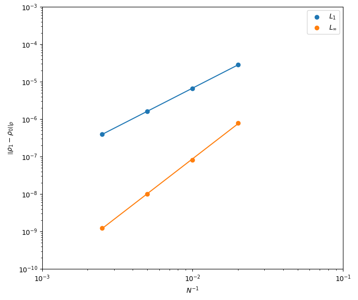
This example case contains an automated convergence test using a 1D, two-component advection case. The case can be run by executing the bash script ./submitJobs.sh in a terminal after enabling execution permissions with chmod +x ./submitJobs.sh and setting the ROOT_DIR and MFC_DIR variables. By default the script runs the case for 6 different grid resolutions with 1st, 3rd, and 5th, order spatial reconstructions. These settings can be modified by editing the variables at the top of the script. You can also run different model equations by setting the ME variable and different Riemann solvers by setting the RS variable.

Once the simulations have been run, you can generate convergence plots with matplotlib by running python3 plot.py in a terminal. This will generate plots of the L1, L2, and Linf error norms and save the results to errors.csv.

Backward Facing Step (2D)

Final Condition (Density)

Shock Droplet (2D)

Reference:

Panchal et. al., A Seven-Equation Diffused Interface Method for Resolved Multiphase Flows, JCP, 475 (2023)

Initial Condition

Result

Taylor-Green Vortex (3D)

Reference:

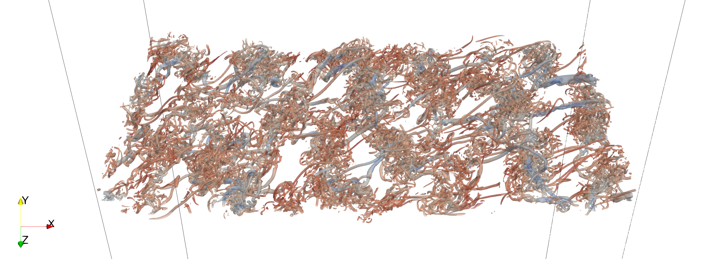
Hillewaert, K. (2013). TestCase C3.5 - DNS of the transition of the Taylor-Green vortex, Re=1600 - Introduction and result summary. 2nd International Workshop on high-order methods for CFD.

Final Condition

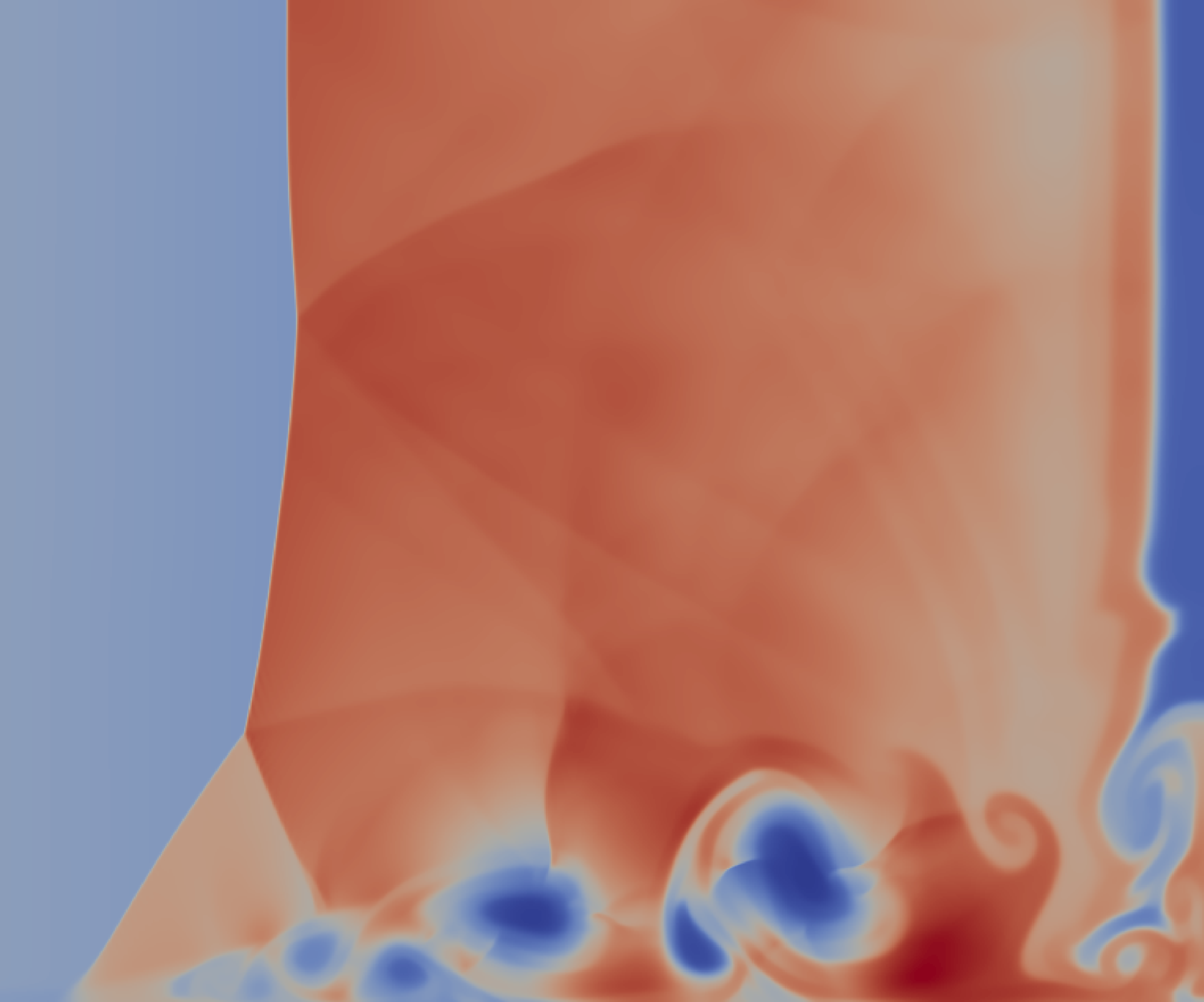
This figure shows the isosurface with zero q-criterion.

Rayleigh-Taylor Instability (2D)

Final Condition and Linear Theory

2D Triple Point (2D)

Reference:

Trojak, W., & Dzanic, T. Positivity-preserving discoutinous spectral element method for compressible multi-species flows. arXiv:2308.02426

Numerical Schlieren at Final Time

3D Turbulent Mixing layer (3D)

Liutex visualization at transitional state

1D Multi-Component Inert Shock Tube

Reference:

P. J. Martínez Ferrer, R. Buttay, G. Lehnasch, and A. Mura, “A detailed verification procedure for compressible reactive multicomponent Navier–Stokes solvers”, Computers & Fluids, vol. 89, pp. 88–110, Jan. 2014. Accessed: Oct. 13, 2024. [Online]. Available: https://doi.org/10.1016/j.compfluid.2013.10.014

Initial Condition

Results

IBM Bow Shock (3D)

Final Condition