|
MFC
Exascale flow solver
|
|
MFC
Exascale flow solver
|
After running post_process on a simulation (see Running), MFC produces output in either Silo-HDF5 format (format=1) or binary format (format=2). These can be visualized using MFC's built-in CLI tool or external tools like ParaView and VisIt.
MFC includes a built-in visualization command that renders images and videos directly from post-processed output — no external GUI tools needed.
The command auto-detects the output format (binary or Silo-HDF5) and dimensionality (1D, 2D, or 3D). By default it launches an interactive terminal UI that works over SSH. Use --interactive for a browser-based UI (supports 3D), --png to save images, or --mp4 for video.
Before plotting, you can inspect what data is available:
The --step argument accepts several formats:
| Format | Example | Description |
|---|---|---|
| Single | --step 1000 | One timestep |
| Range | --step 0:10000:500 | Start:end:stride (inclusive) |
| Last | --step last | Most recent available timestep |
| All | --step all | Every available timestep |
Customize the appearance of plots:
| Option | Description | Default |
|---|---|---|
| --cmap | Matplotlib colormap name | viridis |
| --vmin | Minimum color scale value | auto |
| --vmax | Maximum color scale value | auto |
| --dpi | Image resolution (dots per inch) | 150 |
| --log-scale | Use logarithmic color scale | off |
| --output | Output directory for images | case_dir/viz/ |
For 3D simulations, viz extracts a 2D slice for plotting. By default, it slices at the midplane along the z-axis.
Generate MP4 videos from a range of timesteps:
Videos are saved as case_dir/viz/<varname>.mp4. The color range is automatically computed from the first, middle, and last frames unless --vmin/--vmax are specified.
For 1D cases, omitting --var (or passing --var all) renders all variables in a single tiled figure:
Each variable gets its own subplot with automatic LaTeX-style axis labels. Tiled mode is available for 1D and 2D data. For 3D data, omitting --var auto-selects the first variable.
Launch a browser-based interactive viewer with --interactive:
The interactive viewer provides a Dash web UI with:
The default mode launches a live terminal UI that works over SSH with no browser or port-forwarding needed:
The TUI loads all timesteps and renders plots directly in the terminal using Unicode block characters. It supports 1D and 2D data only (use --interactive for 3D).
Keyboard shortcuts:
| Key | Action |
|---|---|
| . / → | Next timestep |
| , / ← | Previous timestep |
| Space | Toggle autoplay |
| l | Toggle logarithmic scale |
| f | Freeze / unfreeze color range |
| ↑ / ↓ | Select variable (in sidebar) |
| c | Cycle colormap |
| q | Quit |
Axis labels use LaTeX-style math notation — for example, pres is labeled as \(p\), vel1 as \(u\), and alpha1 as \(\alpha_1\). Plots use serif fonts and the Computer Modern math font for consistency with publication figures.
The output format is auto-detected from the case directory. To override:
Run ./mfc.sh viz -h for a full list of options.
ParaView is an open-source interactive parallel visualization and graphical analysis tool for viewing scientific data. Post-processed data in Silo-HDF5 format (format=1) can be opened directly in ParaView. Paraview 5.11.0 has been confirmed to work with the MFC databases for some parallel environments. Nevertheless, the installation and configuration of Paraview can be environment-dependent and are left to the user.
The user can launch Paraview and open the series file /silo_hdf5/collection.silo.series. Once the database is loaded, flow field variables contained in the database can be added to the render view. Further information on Paraview can be found in its documentation. The figure below shows the iso-contour of the liquid void fraction (alpha1) in the database generated by the example case 3D_sphbubcollapse.

Visualizing data in cylindrical coordinates requires a coordinate transformation of the raw data in the database file. In Paraview, this coordinate transformation can be accomplished with the following steps:
These steps will transform the raw data into cylindrical coordinates. For many cases, this step will require resizing the render view window.
VisIt is an alternative open-source interactive parallel visualization and graphical analysis tool for viewing scientific data. Versions of VisIt after 2.6.0 have been confirmed to work with the MFC databases for some parallel environments. Nevertheless, installation and configuration of VisIt can be environment-dependent and are left to the user. Further remarks on parallel flow visualization, analysis, and processing of the MFC database using VisIt can also be found in Coralic [14] and Meng [35].
The user can launch VisIt and open the index files under /silo_hdf5/root. Once the database is loaded, flow field variables contained in the database can be added to the plot. The figure below shows the iso-contour of the liquid void fraction (alpha1) in the database generated by the example case 3D_sphbubcollapse. For analysis and processing of the database using VisIt's capability, the user is encouraged to address VisIt user manual.
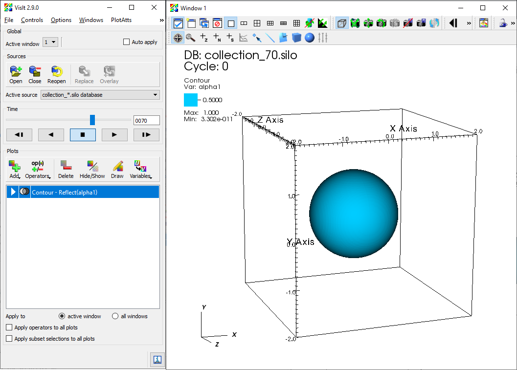
Iso-contour of the liquid void fraction (alpha1) in the database generated by example case 3D_sphbubcollapse
If parallel_io = 'F', MFC will output the conservative variables to a directory D/. If multiple cores are used ( \(\mathtt{ppn > 1}\)), then a separate file is created for each core. If only one coordinate dimension (n = 0 and p = 0) exists, the primitive variables will also be written to D/. The file names correspond to the variables associated with each equation solved by MFC. They are written at every t_step_save time step. The conservative variables are
\[ (\rho \alpha)_{1}, \dots, (\rho\alpha)_{N_c}, \rho u_{1}, \dots, \rho u_{N_d}, E, \alpha_1, \dots, \alpha_{N_c} \]
and the primitive variables are
\[ (\rho \alpha)_1, \dots, (\rho\alpha)_{N_c}, u_1, \dots, u_{N_d}, p, \alpha_1, \dots, \alpha_{N_c} \]
where $N_c$ are the number of components num_fluids and $N_d$ is the number of spatial dimensions. There are exceptions: if model_eqns = 3, then the six-equation model appends these variables with the internal energies of each component. If there are sub-grid bubbles bubbles = T, then the bubble variables are also written. These depend on the bubble dynamics model used. If polytropic = 'T', then the conservative variables are appended by
\[ n_b R_1, n_b \dot{R}_1, \dots, n_b R_{N_b}, n_b \dot{R}_{N_b} \]
where $n_B$ is the bubble number density, and $N_b$ is the number of bubble sizes (see the matching variable in the input file, Nb). The primitive bubble variables do not include $n_B$:
\[ R_1, \dot{R}_1, \dots, R_{N_b}, \dot{R}_{N_b} \]
Begin by downloading the .zip file here. This file contains two things:
Place the file paceParview.zip in your scratch direction on Phoenix and unzip it using unzip paceParaview.zip. Enter the new directory paceParaview and run tar -xvf ParaView-5.11.0-egl-MPI-Linux-Python3.9-x86_64.tar.gz to decompress the compiled binary. Now that you have the binary on Phoenix, you must download Paraview 5.11 on your local machine. Paraview binaries can be downloaded here. Select v5.11 from the version drop-down bar and install a 5.11.0 version of Paraview.
While all of the bash script's options could be passed as command-line arguments, hardcoding certain unlikely-to-change options saves time. The following is a list of required and suggested updates to make to pace-paraview-server.
Before running pace-paraview-server for the first time, you must update its permissions by running chmod u+x pace-paraview-server in your command line. Once this has been done, you can run ./pace-paraview-server with the following options:
Once you run ./pace-paraview-server <options>, it'll take a bit to start up. In the meantime, you'll see the below message:
When initializing is done, you should see a dialogue with some recommended next steps, numbered 1-4. Below is a slightly altered version of that dialogue:
1) Create the appropriate port forwarding for your local ParaView session to connect with.
2) Once you have Paraview5.11.0 on your machine, select File -> Connect.. to open the remote connection dialogue box.